Almost 10 years ago I started developing a web frontend for collectd, Collectd Graph Panel (CGP). A PHP frontend that displays graphs in PNG format using rrdtool and the RRD files created by collectd.
A lot has happened since then. Because of the IoT hype time series databases like Graphite, InfluxDB and TimescaleDB became more popular. Also visualization tools gained more traction, of which Grafana is the most popular one.
In this blogpost I’m going to show a replacement of collectd, RRD files and CGP, by using collectd, InfluxDB and Grafana. I will:
- Hook up collectd to InfluxDB to store the metrics
- Configure InfluxDB to aggregate data over time (it doesn’t do this automatically like RRD)
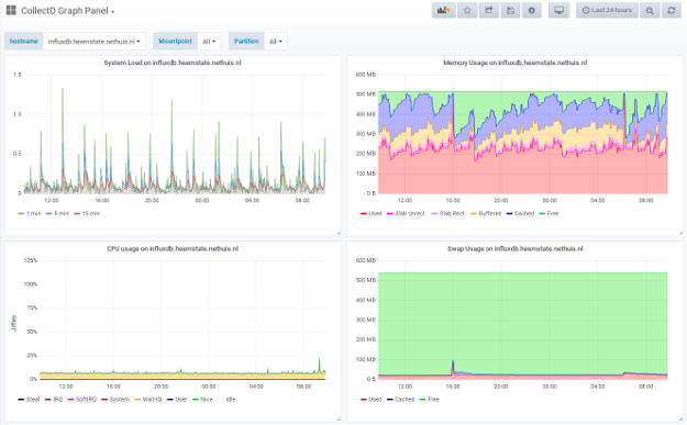
- Use a Grafana dashboard to display the graphs with the same colors and styling I was used to in CGP
Hooking up collectd to InfluxDB
This is pretty simple. First of all follow the installation guide to install the InfluxDB service.
InfluxDB supports the collectd protocol. It can be configured to listen on UDP port 25826, which collectd clients can send metrics to.
I more or less used the default values that were already provided in /etc/influxdb/influxdb.conf:
[[collectd]]
  enabled = true
  bind-address = ":25826"
  database = "collectd"
  retention-policy = ""
  typesdb = "/usr/share/collectd/types.db"
  security-level = "none"
  batch-size = 5000
  batch-pending = 10
  batch-timeout = "10s"
  read-buffer = 0
In the configuration of the collectd clients, InfluxDB can be configured as server in the network plugin:
LoadPlugin network
<Plugin network>
  Server "<InfluxDB-IP-address>" "25826"
</Plugin>
The metrics the collectd clients collect are now send to InfluxDB.
Downsampling data in InfluxDB
Unlike with the RRD files created by collectd, InfluxDB doesn’t come with a default downsampling policy. Metrics are just send by the collectd clients every 10 seconds and saved in InfluxDB and kept indefinitely. You will have super detailed graphs when you for example zoom in on some hourly statistics from 5 months ago, but your InfluxDB data-set will keep growing resulting in gigabytes of data per collectd client.
In my experience for server statistics you want to have detailed graphs for the most recent metrics. This is useful when you want to debug an issue. Older metrics are nice to display weekly, monthly, quarterly or yearly graphs to spot trends. For graphs with these timeframes 10 second metrics are not required. Metrics for these graphs can be aggregated.
In InfluxDB the combination of “Retention Policies” (RPs) and “Continuous Queries” (CQs) can be used to downsample the metrics. One of the things you can define with an RP is for how long InfluxDB keeps the data. CQs automatically and periodically execute pre-defined queries. This can be used to aggregate the metrics to a different RP.
I’ve been fairly happy with the aggregation policy in the RRD files used by collectd. Let’s try to setup the same data aggregation system in InfluxDB.
Information about the aggregation policy can be extracted from the RRD file by using the rrdinfo command. Let’s take for example the cpu-idle.rrd file. This shows that this RRD file contains 1 metric per 10 seconds:
$ rrdinfo cpu-idle.rrd | grep step
step = 10
And this shows the different aggregation policies for the average value of the metrics:
$ rrdinfo cpu-idle.rrd | grep AVERAGE -A6 | egrep '(rows|pdp_per_row)'
rra[0].rows = 1200
rra[0].pdp_per_row = 1
rra[3].rows = 1235
rra[3].pdp_per_row = 7
rra[6].rows = 1210
rra[6].pdp_per_row = 50
rra[9].rows = 1202
rra[9].pdp_per_row = 223
rra[12].rows = 1201
rra[12].pdp_per_row = 2635
There are 5 different aggregations. They all have Primary Data Points per row (pdp_per_row), which means that for example 1 row (metric) is an aggregation of 7 Primary Data Points. And it shows the number of rows that are kept.
Summarized this RRD file contains:
- 1200 metrics of a 10 second interval (12000s of data == 3.33 hours)
- 1235 metrics of a (7*10) 70 second interval (86450s of data =~ 1 day)
- 1210 metrics of a (50*10) 500 second interval (605000s of data == 1 week)
- 1202 metrics of a (223*10) 2230 second interval (2680460s of data == 31 days)
- 1201 metrics of a (2635*10) 26350 second interval (31646350s of data == 366 days)
Let’s connect to our influxdb instance and configure the same using RPs and CQs.
$ influx
Connected to http://localhost:8086 version 1.7.6
InfluxDB shell version: 1.7.6
Enter an InfluxQL query
> show databases
name: databases
name
----
_internal
collect
> use collectd
Using database collectd
> show retention policies
name    duration  shardGroupDuration replicaN default
----    --------  ------------------ -------- -------
autogen 0s        168h0m0s           1        true
The database by default contains the “autogen” RP, with a duration of 0s. No data will be thrown away. First modify the duration of the autogen retention policy to 200 minutes:
> alter retention policy "autogen" on "collectd" duration 200m shard duration 1h
> show retention policies
name    duration  shardGroupDuration replicaN default
----    --------  ------------------ -------- -------
autogen 3h20m0s   1h0m0s             1        true
Now add the additional RPs:
> CREATE RETENTION POLICY "day" ON collectd DURATION 1d REPLICATION 1
> CREATE RETENTION POLICY "week" ON collectd DURATION 7d REPLICATION 1
> CREATE RETENTION POLICY "month" ON collectd DURATION 31d REPLICATION 1
> CREATE RETENTION POLICY "year" ON collectd DURATION 366d REPLICATION 1
> show retention policies
name    duration  shardGroupDuration replicaN default
----    --------  ------------------ -------- -------
autogen 3h20m0s   1h0m0s             1        true
day     24h0m0s   1h0m0s             1        false
week    168h0m0s  24h0m0s            1        false
month   744h0m0s  24h0m0s            1        false
year    8784h0m0s 168h0m0s           1        false
For downsampling in InfluxDB I want to use more logical durations compared to what was in the RRD file:
- 70s -> 60 seconds
- 500s -> 300 seconds (5 minutes)
- 2230s -> 1800 seconds (30 minutes)
- 26350s -> 21600 seconds (6 hours)
These CQs will downsample the data accordingly:
> CREATE CONTINUOUS QUERY "cq_day" ON "collectd" BEGIN SELECT mean(value) as value INTO "collectd"."day".:MEASUREMENT FROM /.*/ GROUP BY time(60s),* END
> CREATE CONTINUOUS QUERY "cq_week" ON "collectd" BEGIN SELECT mean(value) as value INTO "collectd"."week".:MEASUREMENT FROM /.*/ GROUP BY time(300s),* END
> CREATE CONTINUOUS QUERY "cq_month" ON "collectd" BEGIN SELECT mean(value) as value INTO "collectd"."month".:MEASUREMENT FROM /.*/ GROUP BY time(1800s),* END
> CREATE CONTINUOUS QUERY "cq_year" ON "collectd" BEGIN SELECT mean(value) as value INTO "collectd"."year".:MEASUREMENT FROM /.*/ GROUP BY time(21600s),* END
With these CQs and RPs configured you will get 5 data streams: autogen (the default), day, week, month and year. To retrieve the aggregated metrics from a specific RP you have to prefix the measurement in your select query with it. So for example to get the cpu idle metrics you can execute this to get the metrics in the 10s resolution:
> select * from "cpu_value"
# or
> select * from "autogen"."cpu_value"
To get it in 60s resolution (RP “day”):
> select * from "day"."cpu_value"
This is important to know when creating graphs in Grafana. When you want to show a “month” or “year” graph you can not simply do select value from "cpu_value" where type_instance='idle', because you will only get the metrics from the “autogen” RP. You have to explicitly define the RP.
Collectd graphs in Grafana
To install Grafana follow the installation guide.
Create a user in InfluxDB that can be used in Grafana to read data from InfluxDB:
> create user grafana with password <PASSWORD>
> grant read on collectd to grafana
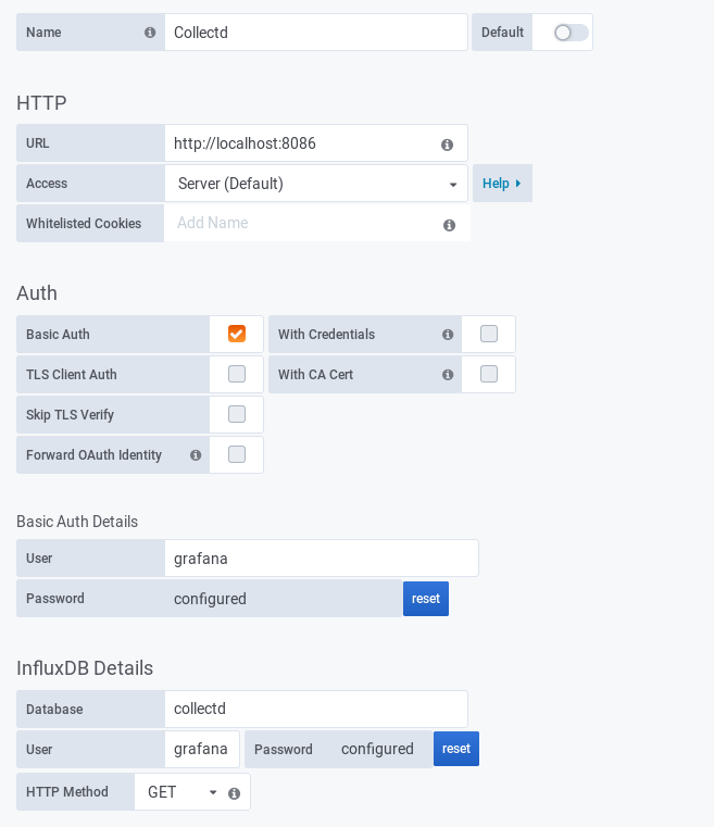
To get access to the collectd data in InfluxDB you need to configure a data source in Grafana:
Now let’s for example create a graph for the load average.
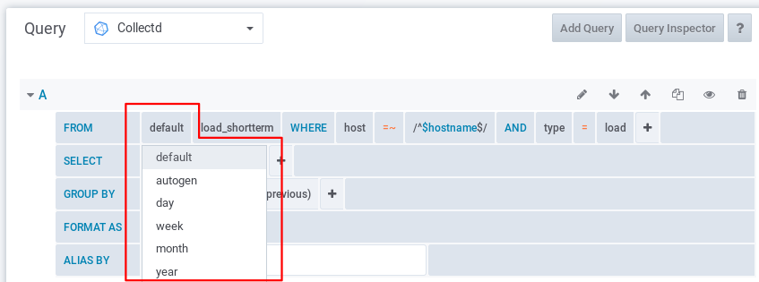
As you can see you have to explicitly select the RP for the metrics you want to display in the graph. There is no easy way to get metrics automatically from all RPs at once. This is of course not really convenient, because once the graph on your dashboard is configured you want to be able to change the time range and just see the data from whatever RP that has the metrics in the most detailed way. So ideally you want the RP to be automatically selected based on the time range that is selected.
There are luckily more people having this issue and Talek found a nice workaround for it.
We can create a variable that executes a query based on the current “From” and “To” time range values in Grafana to find out what the correct RP is. This variable can be refreshed every time the time range changes. The query to find out the correct RP is executed on measurement “rp_config” that has a separate RP (forever) without a duration so this data never gets deleted.
Configure the extra RP and insert the RP data:
CREATE RETENTION POLICY "forever" ON "collectd" DURATION INF REPLICATION 1
INSERT INTO forever rp_config,idx=1 rp="autogen",start=0i,end=12000000i,interval="10s" -9223372036854775806
INSERT INTO forever rp_config,idx=2 rp="day",start=12000000i,end=86401000i,interval="60s" -9223372036854775806
INSERT INTO forever rp_config,idx=3 rp="week",start=86401000i,end=604801000i,interval="300s" -9223372036854775806
INSERT INTO forever rp_config,idx=4 rp="month",start=604801000i,end=2678401000i,interval="1800s" -9223372036854775806
INSERT INTO forever rp_config,idx=5 rp="year",start=2678401000i,end=31622401000i,interval="21600s" -9223372036854775806
In the start and end times I added one extra second (86400000i -> 86401000i) because I noticed when for example selecting the “Last 24 hours” range in Grafana, $__to – $__from never was exactly 86400000 milliseconds.
Create the variable in Grafana:
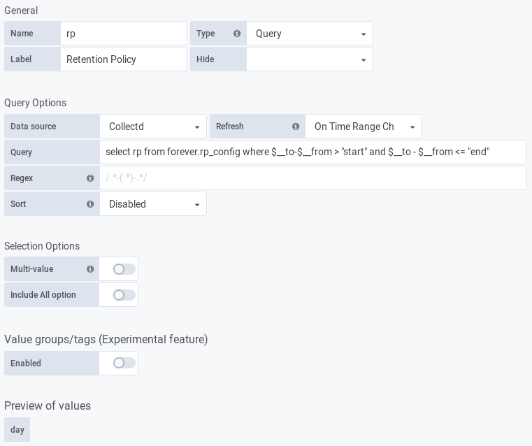
And use the $rp variable as RP in the queries to create the graph:
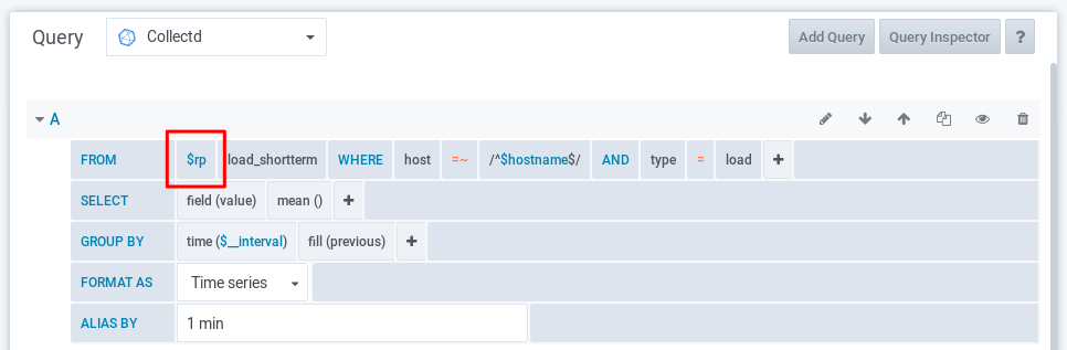
There is one caveat with this solution. It only works when the end of the time range is now (current time), for example by selecting a “Quick range” that starts with “Last …”. The query only looks at how long the time range is. Not if the RP contains the full time range. I’ve not been able to achieve this by using the available variables in Grafana like $__from, $__to and $__timeFilter and the possibilities that InfluxQL has. I’ve tried to adjust the query to do something like select rp from rp_config where $__from > now() - "end", but that is not supported by InfluxDB and returns an empty result.
The effect of the caveat is that when you zoom in on older metrics, the $rp variable will select an RP that does not contain the data anymore. When changing the $rp variable manually you can see that less detailed metrics are available in different RPs. For example:
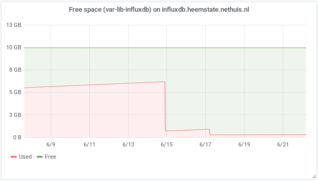
Result: Less storage required
I monitor 6 systems with collectd in my small home-setup. After configuring the collectd clients to send the metrics to InfluxDB and running this setup without RPs and CQs for a couple of weeks it already required 6 gigabyte of storage. After configuring the RPs and CQs the collectd InfluxDB now uses 72 MB. The RRD files in my previous setup used ~186 MB for these 6 systems.
Grafana Dashboard available
To make things easy I’ve already created a dashboard that uses the same colors and styling as Collectd Graph Panel. It can be downloaded here: https://grafana.com/dashboards/10179